Why Millimeter Wave Requires a Different Approach to DPD and How to Quantify Its Value

Hossein Yektaii, Patrick Pratt, and Frank Kearney, Analog Devices

In the 5G New Radio standard, millimeter wave (mmWave) frequencies, in addition to sub-6 GHz frequencies, are utilized to enhance throughput. The use of mmWave frequencies provides unique opportunities for a drastic increase in data throughput while presenting new implementation challenges. This article explores architectural differences between sub-6 GHz and mmWave base station radios, with particular emphasis on the challenges and benefits of implementing DPD on these systems. While digital predistortion (DPD) is a well-established technique commonly used in sub-6 GHz wireless communication systems to improve the power efficacy, most mmWave radios do not use DPD. Using a prototype 256 element mmWave array, built with ADI beamformers and transceivers, we are able to demonstrate that DPD improves the effective isotropic radiated power (EIRP) by up to 3 dB. This allows for a 30% reduction in the number of array elements, relative to an array without DPD, for the same target EIRP.

The purpose of this article is to draw a comparison between a traditional sub-6 GHz macrocellular and a mmWave base station radio and antenna design. It further covers how these design differences impact DPD implementation in mmWave arrays relative to sub-6 GHz radios.

Introduction

In addition to reduced latency and higher reliability, the exponential increase in demand for higher data throughput has been one of the most powerful driving forces behind 3GPP 5G NR standard. While the 4G LTE systems were deployed in sub-3 GHz bands, the allocation of the new spectrum in the 3 GHz to 5 GHz range in recent years has enabled wider channel bandwidths (BW) in 5G NR. Compared to the 4G LTE, the maximum channel bandwidth has increased from 20 MHz to 100 MHz in sub-6 GHz frequencies. Besides wider channel BW, multiple transmit and receive antennas and ultimately massive MIMO technology has further increased the spectral efficiency. While all these improvements help to deliver higher data throughputs, the fundamental limitation—the relatively small amount of allocated sub-6 GHz spectrum—continues to limit the peak throughput for individual users to less than 1 Gbps.

In 5G NR, for the first time in the history of the 3GPP standards, millimeter wave frequencies between 24.25 GHz to 52.6 GHz are allocated for cellular mobile applications. This new frequency range is referred to as FR2 in contrast to the sub-6 GHz frequencies termed FR1. There are much larger swaths of spectrum available in FR2 relative to FR1. A single channel in FR2 could be as large as 400 MHz, enabling unprecedented throughput. However, the use of mmWave frequencies brings new implementation challenges to both the base station (BS) and user equipment (UE). The most significant of these challenges are higher path losses and lower PA output powers, making the link budget between the base station and UE quite challenging.

Path loss between BS and UE is defined as Pl [dB] = 10log10 (Pt/Pr), where Pt and Pr are the transmitted and received power, respectively. In free space, the received power is a function of distance and wavelength, also known as Friis’ formula, where Pr(d,λ) = Pt Gt Gr (λ/4πd)², and Gt and Gr are the transmitter and receiver antenna gains, respectively. λ is the wavelength and d the distance between transmitter and receiver. In a typical wireless communication environment, due to reflection off nearby objects and loss through construction material, the path loss is much more complex to model and estimate. However, to form an understanding of higher path loss at mmWave frequencies compared to sub-6 GHz, let us assume free space propagation, similar antenna gains, and equal distances between BS and UE. Using this approach, the path loss at 28 GHz compared to 900 MHz is 10xlog(28000/900)² = 29.8 dB higher!

It is not uncommon for BS power amplifiers at sub-6 GHz frequencies to output tens of watts of RF power with efficiencies above 40%. This is enabled by the adoption of high efficiency PA architectures such as Doherty and the use of advanced digital predistortion techniques. In contrast, the highly linear class AB mmWave PAs typically output less than 1 W of RF power and have single digit efficiencies. At mmWave frequencies, these operating conditions exacerbate the link budget challenges between BS and UE. The solution to both challenges—the larger path loss and lower power per PA—is the more accurate delivery of power to specific spatial locations. This is achieved using active phased array antennas that offer beamforming and beamsteering capabilities.

Antenna Arrays in mmWave 5G

Antenna arrays are not a new concept. Passive arrays have been used in cellular base station antennas since the early years of the GSM deployment, and radar systems have been using them for several decades. As stated in the previous section, the solution to larger path loss and lower power per PA in mmWave frequencies is to use active phased array antennas. This is achieved by placing many antenna elements in an array, while each element is driven with a low power PA. Using more elements increases the total radiated power out of the array and at the same time enhances the array gain and narrows the resulting beam. The phased array antenna theory is beyond the scope of this article. For further information on the topic please refer to the three-part Analog Dialog series, “Phased Array Antenna Patterns.”1-3

The high cost of active phased array antennas has limited their application mostly to aerospace and defense applications. More recent advances in semiconductor technology, combined with high levels of integration, have made it possible for active phased array antennas to become commercially viable in 5G applications. ADI offers active beamformer devices that integrate 16 complete transmit and receive channels with associated PAs and low noise amplifiers (LNAs), as well as per path phase and gain controls and TDD switch functionality. All this integrated on a single piece of silicon! The first generation of these devices were implemented using SiGe BiCMOS technology (ADMV4821). To further improve the power efficiency and cost, the second generation uses the SOI CMOS process (ADMV4828). These highly integrated and power efficient beamformers, along with mmWave up/downconverters (ADMV1017/ADMV1018) and frequency synthesizers (ADF4371/ADF4372), enable a complete RF front-end solution for mmWave 5G base stations.

At mmWave frequencies, the antenna elements have a small physical footprint. For example, a simple microstrip patch antenna at 28 GHz is typically smaller than 10 mm2. Therefore, many antennas can be placed in a relatively small area to enhance the gain. Let’s assume a 256 element antenna array with eight rows and 16 columns of dual polarized radiating elements, as shown in Figure 1. The red and blue lines indicate +45° and –45° polarized elements, respectively.

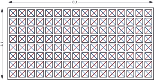
Figure 1. A 256 element antenna array with dual polarized radiating elements.

The total area of such antenna array, assuming λ/2 distance between antenna elements, is 8(λ/2) × 16(λ/2) = 32λ2. Comparing a 900 MHz and a 28 GHz antenna, the total area of a 900 MHz array is 3.55 m2, whereas the 28 GHz array is only 3.67 × 10-3 m2—almost 1000 times smaller! While the size of a 256 element antenna array at 900 MHz is quite prohibitive, a similar array at 28 GHz can be implemented on a printed circuit board (PCB) in an area less than 40 square centimeters.

A 256 element dual polarized mmWave antenna array at 28 GHz was developed on a multilayer PCB, using ADI beamformers and mmWave up/downconverters. To reduce the cost and avoid expensive/lossy interconnect between antenna and radio, active components where mounted on one side and the antenna elements on the other side of the PCB. A picture of this board, which is called AiB256 (AiB stands for antenna in board), is shown in Figure 2.

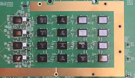
Figure 2. The component side of AiB256 (16 beamformers and four mmWave up/downconverters).

There are 16 ADMV4828 SOI beamformer chips on AiB256, each providing 16 transmit and 16 receive channels, connecting to 128 antenna elements in each polarization, covering a frequency range of 26.5 GHz to 29.5 GHz. Each of the 64 antenna elements of the same polarization are connected to a separate ADMV1018 mmWave up/downconverter. Therefore, a total of four independent beams can be formed. A simplified block diagram for half of the AiB256 is shown in Figure 3.

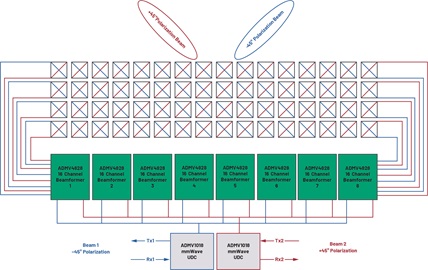
Figure 3. Functional block diagram for half of AiB256 (not all the interconnects shown).

To get to higher EIRP, two sets of 64 antenna elements of the same polarization could be combined at IF to generate a total of two beams, with 128 antenna elements forming each beam. This board was used extensively to support the development of antenna calibration and DPD algorithms in house.

Base Station Design for Sub-6 GHz and mmWave

When designing a base station at a given frequency and desired coverage area, often the beam pattern and effective isotropic radiated power (EIRP) are specified as a prerequisite. A typical macrocellular base station at 900 MHz consists of a 4Tx/4Rx radio unit (RU) and is connected to an external antenna, as shown in Figure 4.

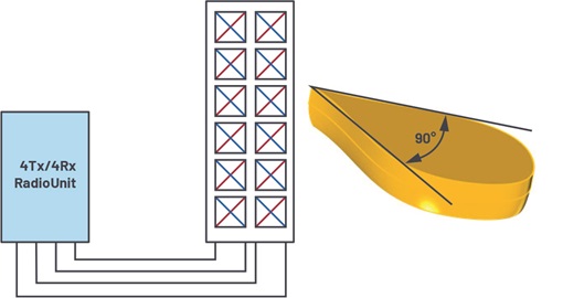
Figure 4. A 900 MHz base station with a 4Tx/4Rx radio unit and dual polarized two column antenna.

Inside the antenna there are two columns of cross polarized (±45° red/blue) dipoles. Each of the four RF ports feeds one polarization on one column. In this example, the signal is split with equal phase and amplitude between the six dipoles of the same polarization. Having a larger number of elements in the vertical direction (columns) squeezes the beam in the vertical plane (see Figure 4). This is desirable because most of the UEs are below the antenna height. There is often some amount of beam down-tilting to further limit the cell coverage area and avoid interference with other cells. Assuming λ/2 spacing between the antenna elements, the half power beam width (the angle where the transmit power drops by 3 dB relative to the peak of the beam) of such antenna is typically around 90° in the horizontal plane and less than 20° in the vertical plane. This wide beam covers a typical 120° sector and does not need to be steered to track the UE movement. The antenna height and width are 6 × (λ/2) = 2 meters and 2 × (λ/2) = 0.33 meters, respectively. The gain of the antenna for each polarization, assuming 5 dBi gain per dipole element, is approximately 10 × log(12) + 5 dBi = 15.8 dBi. If each PA puts out 40 W (46 dBm) of RF power, the EIRP per polarization is 46 dBm + 3 dB (2 columns) + 15.8 dBi = 64.8 dBm. This level of EIRP would be expected to provide good coverage over distances of several kilometers at 900 MHz.

Now let’s consider the 28 GHz AiB256 with 128 antenna elements per polarization arranged in eight rows and 16 columns, as shown in Figure 1. Assuming λ/2 distance between the elements and 5 dBi gain per element, the overall antenna gain is approximately calculated as 10 × log(128) + 5 dBi = 26 dBi. Compared to the 900 MHz example, the antenna gain is 10.2 dB higher. However, this comes at the expense of narrower beam width. The 3 dB beam width is only 12° in the vertical plane and 6° in the horizontal plane. Such a narrow beam is not able to cover a typical 120° sector all at once. The solution is to first find the active UEs in the cell coverage area, point the beam to them and track their movement in the cell. The 5G standards specify the beam acquisition and tracking procedures, which is outside the scope of this article. To calculate the EIRP of this radio, let’s assume each transmit path puts out 13 dBm of RF power. The total power per polarization is 13 dBm + 10 × log(128) = 34 dBm. Combined with 26 dBi antenna gain, the total EIRP per polarization is 34 dBm + 26 dBi = 60 dBm. In a typical outdoor deployment scenario, this level of EIRP covers up to a few hundred meters at 28 GHz.

Value of the DPD in Sub-6 GHz Systems

5G and 4G wireless standards are based on OFDM signals with an inherently high peak-to-average power ratio (PAPR). To amplify and transmit these signals with high fidelity and to avoid polluting the adjacent channels, care must be taken not to compress or clip the signal peaks. This requires operating the PA at average power levels 6 dB to 9 dB below its peak power capability. Operating the PA in such deep back-off regime results in very low efficiency, often less than 10%.

Efficient PA architectures such as Doherty maintain high efficiency across 6 to 9 dB below their peak power, but they are considerably less linear compared to class AB PAs. If deployed without any linearization technique, they fail to meet the error vector magnitude (EVM) and adjacent channel power ratio (ACPR) required by the application. One of the most popular linearization techniques is DPD, which is widely used in sub-6 GHz systems.

Sub-6 GHz systems require the EVM to be less than 8% and 3.5% for 64-QAM and 256-QAM modulations, respectively, for 3GPP standard 38.104.1 To meet these EVM requirements the PAPR of the signal should be maintained between 6 dB to 9 dB. The ACPR should normally be less than –45 dBc for 3GPP standard 38.104. In the previous example of a 900 MHz 4Tx/4Rx radio with 40 W of rms output power per transmitter, if the power amplifiers are to be operated in linear region to meet the EVM and ACPR requirements, their efficiency is normally less than 10%. This means each of the four PAs consume more than 400 W of DC power to put out 40 W of RF power. Therefore, just the four PAs alone consume more than 1600 W! This has huge implications on the size, cooling, reliability, and operating expenses (OPEX) of the radio. In contrast, using a Doherty PA in combination with the crest factor reduction (CFR) and DPD techniques results in PA efficiencies greater than 40%. This means that each PA consumes less than 100 W of DC power to put out 40 W of RF power. The four PAs in the radio consume less than 400 W of DC power. The rest of the radio normally consumes less than 50 W of DC power. Therefore, the PA power consumption makes up more than 85% of the total DC power consumed by the radio, even when Doherty amplifiers with DPD and CFR are deployed.

Implementation and Value of the DPD in mmWave Arrays

n the AiB256, there are 256 transmit and receive chains capable of generating two or four beams with 128 or 64 PAs deployed in each beam. Like sub-6 GHz systems, the EVM requirements for the mmWave bands are 8% and 3.5% for 64-QAM and 256-QAM modulations, respectively. However, the ACPR requirements in mmWave are much less stringent than sub-6 GHz; they are 28 dBc for 28 GHz band and 26 dBc for 39 GHz band in 3GPP standard 38.104.

Each class AB PA in an ADMV4828 beamformer can deliver 21 dBm of peak power. Operating the PAs on ADMV4828 at approximately 12 dBm rms output power leaves 9 dB headroom to the peak power and results in both the EVM and ACPR requirements being achieved. At 12 dBm (16 mW) output power, each transmit chain consumes around 300 mW of power, resulting in 5% efficiency. Some of the power in the transmit chain is consumed by the variable phase shifters that are necessary for beamforming. Each receive path, including the variable phase shifters, consumes around 125 mW of DC power.

Based on the above power numbers, it is clear that the share of the PA power consumption in a mmWave radio relative to the total DC power consumption is much smaller compared to a sub-6 GHz radio. This raises the question of whether a mmWave radio could still benefit from the DPD or not?

To answer this question, one needs to propose a suitable DPD architecture in mmWave. Simple extension of the DPD implementation form sub-6 GHz systems to mmWave, requires a DPD loop around every one of the PAs. In our AiB256 example, that would mean 256 DPD loops! Obviously, implementing 256 DPD loops is very expensive and power hungry. Since each PA puts out a small amount of power (12 dBm typical), the overall system efficiency with DPD is most likely less than a system without DPD.

Fortunately, there is an elegant solution to this problem. AiB256 could put out a maximum of four beams using 64 PAs in each beam (Figure 3). That means each PA gets the same signal as the other 63 PAs, except for a relative phase shift that is applied for beamsteering. If a single DPD loop is wrapped around the cluster of 64 PAs, then we only need a total of four DPD loops for the entire AiB256 array. Essentially, the DPD loop is wrapped around each beam as opposed to each PA. We refer to this as an array DPD to distinguish it from sub-6 GHz DPD, which has a dedicated DPD loop per PA.

The observation receiver must “look” into the boresight of the beam, where the signals from all PAs add in-phase, so it can correct the distortion caused by the cumulative far-field aggregation of 64 PAs. Our early stage evaluation used a far-field horn antenna as the DPD observation receiver, as shown in Figure 5, and demonstrated that a single DPD loop could be wrapped around a beam to improve the EVM and ACPR. Future ADI products may include an integrated observation path to simplify the DPD implementation.

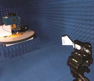
Figure 5. Far-field horn antenna as DPD observation receiver.

The DPD setup uses ADRV9029 integrated transceivers with built-in CFR and DPD capabilities for signals up to 200 MHz bandwidth. Future ADI transceivers will support at least 400 MHz of BW with DPD.

Our analysis found that mmWave array DPD can boost the beam EIRP by more than 3 dB (in a range of 1.5 dB to 3.2 dB) over the frequency range of 26.5 GHz to 29.5 GHz. Optimizing the output matching and bias settings of the beamformer at specific frequencies can result in up to 13 dBm rms output power, while maintaining EVM and ACPR specifications. However, it is not possible to maintain this level of performance across a wide range of frequencies and multiple units. Alternatively, if the appropriate conditions are met (the saturated power level of the PA is maintained above 21 dBm), the use of DPD consistently achieves an output power of more than 14 dBm across the band of interest.

When specifying a mmWave array, the EIRP per beam is a core requirement. If the power per element is relatively small, many elements are needed to achieve the target EIRP, which in turn increases the cost, power, and the size of the array. The more elements deployed in the array, the narrower the resulting beam. Narrower beams are not always desirable; they make pointing the beam and tracking the mobile users more challenging. The plot in Figure 6 illustrates how the number of required elements and the array DC power consumption change as a function of DPD improvement from 0 dB to 3 dB, while maintaining a target EIRP of 60 dBm.

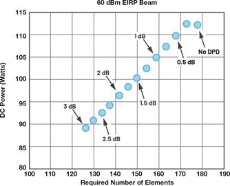
Figure 6. Required number of elements and DC power as a function of DPD improvement.

If 3 dB EIRP improvement is achieved by applying the DPD, the number of required elements is reduced by almost 30% and the power dissipation drops by about 20%. Compared to our sub-6 GHz example, where applying the DPD reduces the power consumption of the PAs by a factor of 4, the power savings in the mmWave array is not as significant. However, in the case of mmWave, we get an additional dividend in that the 30% reduction in the number of elements represents a considerable saving in the cost and size of the array hardware. In the future, it is possible to use more efficient PA architectures in mmWave beamformers to further improve the power efficiency with DPD.

Conclusion

DPD implementation in 5G mmWave arrays brings new challenges relative to sub-6 GHz frequencies. Wrapping a DPD loop around the beam, as opposed to individual PAs that form a beam, makes array DPD feasible and beneficial. Our analysis has shown that there are tangible benefits in terms of higher output powers, system power saving, and hardware reduction. We would, however, urge caution: mmWave DPD in both its application and its evaluation needs to be viewed through a different perspective than that of legacy sub-6 GHz. As mmWave PA architectures mature, that positioning may shift, but for now we need to reinvent the application of DPD as well as our positioning on the benefits.

References

1 38.104: Base Station (BS) Radio Transmission and Reception. 3GPP, March 2017.

Delos, Peter, Bob Broughton, and Jon Kraft. “Phased Array Antenna Patterns— Part 1: Linear Beam Array Characteristics and Array Factor.” Analog Dialogue, Vol. 54, No. 2, May 2020.

Delos, Peter, Bob Broughton, and Jon Kraft. “Phased Array Antenna Patterns— Part 2: Grating Lobes and Beam Squint.” Analog Dialogue, Vol. 54, No. 2, June 2020.

Delos, Peter, Bob Broughton, and Jon Kraft. “Phased Array Antenna Patterns— Part 3: Sidelobes and Tapering.” Analog Dialogue, Vol. 54, No. 3, July 2020.

Authors

Hossein Yektaii began his career at Analog Devices in November 2016. Before joining ADI, he worked at Nortel, Alcatel-Lucent, and Nokia, where he held different positions ranging from RF design engineer to radio system designer. In his current role as a wireless system architect, he leverages his end-to-end radio system knowledge to better understand customer requirements and shape the architecture and specifications of increasingly sophisticated ADI solutions in the wireless market. He studied electrical engineering at Sharif University of Technology and received his master’s degree in telecommunications from Tehran University.

Patrick Pratt is a senior research scientist in the Communication System Team of Analog Devices. His career spans over 30 years and encompasses algorithm research and development activity, both in private organizations and academic institutions. Patrick holds a Ph.D. in electronic engineering from Cork Institute of Technology.

Frank Kearney joined Analog Devices after graduation in 1988. During his time with the company, he has held a diversity of engineering and management roles. He currently manages a team of architects and algorithm developers in the Wireless Systems Group. The group’s focus is on transmit path efficiency and system-level enhancements for O-RAN radio architectures. Frank holds a doctorate from University College Dublin.

Source