What Are Oscilloscopes?

If you’re reading this, you are probably new to the idea or considering buying your first oscilloscope. So what is an oscilloscope? The name has it all: oscillo – to oscillate (vary up and down) and scope – to see. In other words, it’s a tool or you to see electrical signals which change in amplitude with time.

The Right Oscilloscope for You

There are many types of scopes (we’ll call them that for now)— analog, cathode ray tube (CRT)-based, digital, LCD, PC adapters. Scopes are ancient by electronic timeline standards and first appeared in WW2 to help develop the first radar system, but they have stayed the course and have come a long way since then. But for this article, we will stick to an analog, CRT-based scope because if you are considering getting one, this will be your most cost-effective route. Many second-hand perfectly functional ones are readily available out there.

Excellent second-hand buys would include Tektronix, HP (Agilent) Kikosui, and National. The higher the scope’s bandwidth (the maximum frequency it will display accurately), the more you will pay. For general purpose use, 20MHz will suffice, but 100MHz is better if you want to work on RF stuff. Get the highest you can afford. But if you are a beginner, a very complex, expensive scope will just frustrate you. Don’t worry about a delayed timebase—in my 40 years of using scopes, I may have needed this three or four times.

Shown below are three scopes in my lab. I use all of them as they each have their own characteristics and usefulness. These are a digital Tektronix, an analog Kikosui, and an analog Philips with delayed timebase (left to right). In general, digital scopes are great for displaying measured values but trigger poorly or alias when looking at complex RF wave-forms like modulated signals, whereas analog scopes excel here.

What is it for?

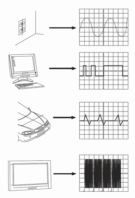
Why would you want to use a scope rather than a multimeter? It’s because the scope can see beyond the numbers on a multimeter LCD. The scope virtually enables you to “see” electric signals, both DC and AC. In a nutshell, it shows changes in voltage against time. So if you connect it to a sine-wave source, you will see a sine wave on the screen and the relationships of different wave-forms to each other, such as phase and frequency. Major uses include the following:

• Observing signals at various points in an amplifier to look for distortion, clipping, and offset;
• Looking at digital circuits to check on shape and level of pulses, perhaps unwanted glitches, seeing that oscillators are running cleanly and at the right frequency; and
• Looking at the output levels of transducers guitars, microphones, etc.

What’s inside and how does it work?

This article is not about designing the innards of a scope. But in a nutshell, there is a long valve-like CRT with a heated cathode at the far end, and the screen end is the anode (with a phosphorus coating) with a super high voltage applied to it (thousands of volts, so keep your hands out of there!). This high voltage causes a stream of electrons to leave the cathode and hit the anode (screen), causing it to fluoresce (glow) at the spot they hit. On either side of the tube’s neck are two sets of deflection plates, X and Y. If you apply a potential to these, they cause the beam to deflect and the spot to move off the center. So if you apply an AC voltage to the Y plates (vertical), you would get a vertical line on the screen. Conversely, if you did the same to the X plates (horizontal), you would get a horizontal line. You can see that applying signals to both will get you some graph on the screen with a bit of imagination.

If we add a few more circuit parts—an amplifier/attenuator to control the Y input signal levels, a time base ramp oscillator to apply to the X plates and cause them to create a horizontal sweep and a way of syncing this to the input frequency and phase—you will have a basic oscilloscope. The screen will have graticules on it, and both the X and Y amplifiers will have calibrated control knobs to show the vertical deflection in volt/division and horizontal in µS an mS per division.

Never open your scope unless you are a trained scope service technician. There are lethal voltages inside. Also, never connect your scope probes to the AC mains unless you know what you are doing. Getting this wrong may kill the scope and you. It can be done using an isolation transformer and possible differential probes, but this is an advanced topic.

Setting up the Scope

This is not as simple as it sounds: when you are first confronted with an unfamiliar scope that has all its knobs twiddled, it may take you several minutes to get a display back on the screen. So here is a brief way to navigate this:

1. Make sure that the scope is turned on—either a led, pilot lamp, or the graticule should light.
2. Turn all the knobs to the central position.
3. Turn the intensity knob to about 80%.
4. Select ‘auto’ in the sweep selection.
5. Select ‘internal’ in the sweep source.
6. Set triggering to channel 1 internal.
7. Vertical mode selects channel 1 and selects AC coupling.
8. Vertical set to 0.1V/div.
9. Horizontal set to 1mS/div.

Twiddle the vertical and horizontal position knobs to see if you can find the trace. The scope should now be showing a horizontal line. If you have a trace, adjust the focus and intensity.

Connect a probe and touch the tip. You should see a rough mains 50Hz waveform, adjust the vertical and horizontal controls to get a display that fits the screen.

If your scope has a calibrator, connect the probe to that, and you should get a nice clean square wave, usually 1V or 5V, at 1kHz. If it is over or under shooting, adjust the small trimmer on the probe for a nice clean square wave.

You are now good to go.

NOTE: If possible, use the 10X setting on the probe if it has one, for wider bandwidth. There are many options to look at now, which channel to trigger on (the one your probe is connected to), and you may need to adjust a hold-off knob if there is one to get a stable display. If you have a dual-channel scope, there are some options like ALT CHOP and ADD. ADD displays a single trace, which is the arithmetic sum of both channels. ALT displays a full sweep of channel 1 then a full sweep of channel 2. CHOP does something similar but displays a bit of each trace alternately. You will have to play with ALT and CHOP to get the best display for the sweep frequency and triggering you are using. We never mentioned DC measurements. If you set the vertical coupling to DC, you can use the vertical position to set a baseline and then do DC measurements. I highly recommend this as you may get unexpected results like an excessive ripple on a power supply, an AC signal at a point where you expected DC, something oscillating, stray spikes and pulses. If I have a fault or something just does not work, I check the DC conditions, and I always do that with a scope.

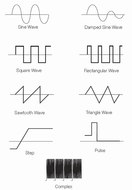
Some examples of waveforms

(Used with permission from Tektronix)

Some real measurements

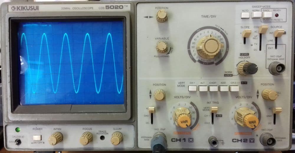
In the scope image below, there is a nice clean sine wave on the screen and we are going to find the amplitude and frequency.

To find the amplitude, you need to know 3 things: the probe gain (X1 or X10), the vertical amplifier volts/div, and the size of the wave-form on the screen. So in the image above, probe gain is X1, volts/div is 50mV/div and the wave form is 6 divisions. Given that, the peak to peak voltage (Vpp) is 50*6 = 300mVpp. The peak value is half of that—150mV and the RMS value (what you would read on a meter) is 0.707*150 = 106mV (0.707 is 1/√2).

To find the frequency (F), we only need the time/div and the number of divisions between any two repeating wave-form peaks. In the example below, time/div is 0.5mS.div and there are 2.2 div 0.5*10-³ = 0.0011. Now, this is the period, and F is 1/period = 1/0.0011 = 909Hz.

Other measurements

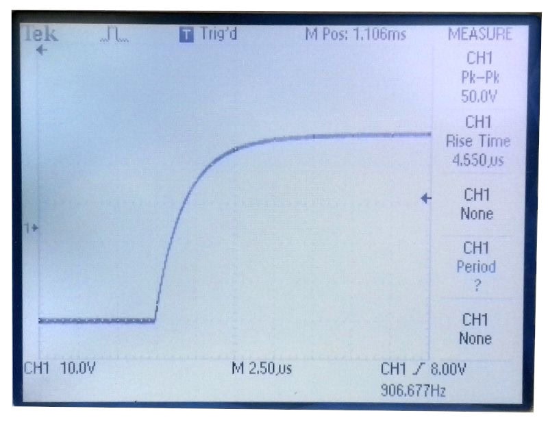
Rise time is defined as the time required for a pulse to rise from 10 percent to 90 percent of its steady value. The rise time shown is 4.55uS. Doing this manually in the trace, the horizontal time/div is 2.5uS/div, and it looks like it took about 1.8 divisions, i.e., 1.8*2.5uS = 4.5uS.

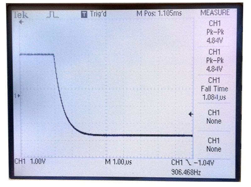
Fall time is defined as the time required for a pulse to fall from 90 percent to 10 percent of its steady value. In the trace shown, the horizontal time/div is 1uS, and if you didn’t have the fancy scope (shows 1.08uS), you could estimate it at about 1 div, i.e., 1uS.

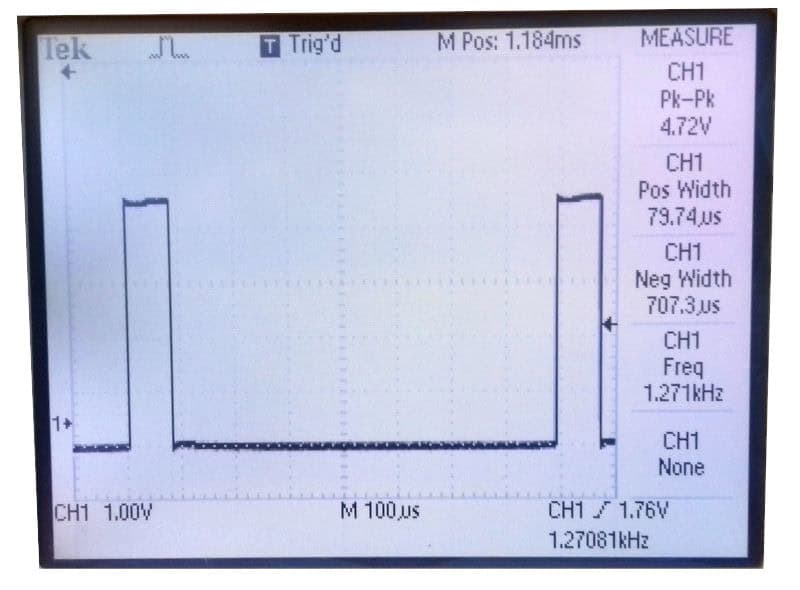
The duty cycle is the ratio of pulse duration or pulse width (PW) to the waveform’s total period, expressed as a percentage. In the example, the frequency is 1.3kHz, so the period is 1/f = 786uS, and the pulse high time is 79.7. The duty cycle is 79.7/786 = 10.1%. You could also estimate this as follows: the horizontal is 100uS/div and about 8.8 divs, and the pulse looks about 90uS wide, so the duty cycle is 90/(8.8*100) = 0.1023, 10.2%, which checks.

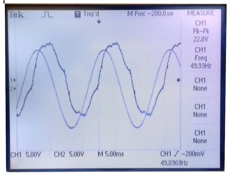
Phase measurement. Here is a 50Hz trace (the rough one) and a signal generator set to almost the same frequency, but offset in phase (the clean sine-wave). Note that the signal generator is leading the 50Hz by about 1 division ie 5mS. Phase θ = td * F * 360° =5mS*50*360 = 90° leading.

You can do a great deal with an oscilloscope, considerably more than what a multimeter could offer. It is a pretty powerful and sophisticated tool, and it will be worth your while to get/download its manual and study it carefully. If I had to set up a minimalist electronics workbench, it would consist of a solder station, a multimeter, a variable power supply, and, definitely, a scope!

Source